Water in modern games
How do modern games render water, I always asked myself? In this blog post I am going to explain the deep secrets of how big studios render water in detail. There are a lot of aspects and ways to make use of water so to make it a little simpler to follow I am going to focus on oceans in specific. Do keep in mind that this is not a tutorial, since the implementation is written in a custom ps5 engine I made in my second year of studying at Breda university of applied sciences.
So let’s start at the beginning by looking at a couple implementations of games that make great use of an ocean.
Horizon forbidden west swimming through a rough ocean
Sea of thieves ocean with light scattering through the waves
The big question is how can we achieve this?
What do we need
There are 2 major components that we need to create a realistic looking ocean the first component is an oceanographic spectra and the second component is the fast Fourier transform which I will explain later on in this post.
Setting up the energy spectrum
So what is this Oceanographic spectra? It is formula that simulates ocean waves under certain conditions, these waves are produced by different wind speeds over big areas and gravity lowers the wave amplitudes. Luckily for us we don’t have to get the data from these ocean ourselves since other people did the work for us. I decided to use the JONSWAP (Joint North Sea Wave Project) spectrum for my implementation since it has a lot of artistical control and is based of accurate data of the north sea.
JONSWAP formula
\[S(\omega) = \frac{\alpha g^2}{\omega^5} \exp\left[-\beta \frac{\omega_p^4}{\omega^4}\right] \gamma^a\]Where:
$a = \exp \left[ -\frac{\left( \omega - \omega_p \right)^2}{2 \omega_p^2 \sigma^2} \right]$
$\sigma = \begin{cases} 0.07 & \text{if } \omega \leq \omega_p \ 0.09 & \text{if } \omega > \omega_p \end{cases}$
$\beta = \frac{5}{4}$
- α is a constant that relates to the wind speed and fetch length. Typical values in the northern North Sea are in the range of 0.0081 to 0.01.
- ω is the wave frequency.
- ωₚ is the peak wave-frequency.
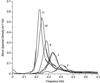
JONSWAP spectra wave amplitude at certain frequency
Now that we have our energy spectrum function we want to randomly sample it and put all the data into a texture this is done with the formula:
\[\hat{h}_0(k) = \frac{1}{\sqrt{2}} (\xi_r + \xi_i) \sqrt{P(k)}\]| $p(k)$ | Is the Wave energy spectrum of choice |
| (ξr+ξi) | are the Gaussian distributed real and imaginary random numbers |
We run this formula for every pixel of the texture so performance scales depending how detailed you want the waves to look, I am using a 512x512 texture since this is perfect for real-time games. The output of this will look something relatively close to this texture depending on what energy spectrum you used.
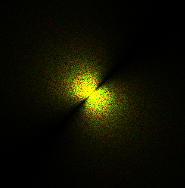
The origin of the spectrum is in the center, the distance from the origin is the frequency, the pixels value is the amplitude and the direction from the origin to the pixel is the direction of the wave.
The energy spectrum texture only has to be computed once unless you change the parameters, but if we want our waves to move we have to update the spectrum by multiplying it with Euler’s formula.
\[\hat{h}(k,t) = \hat{h}_o(k) * e^{it}\]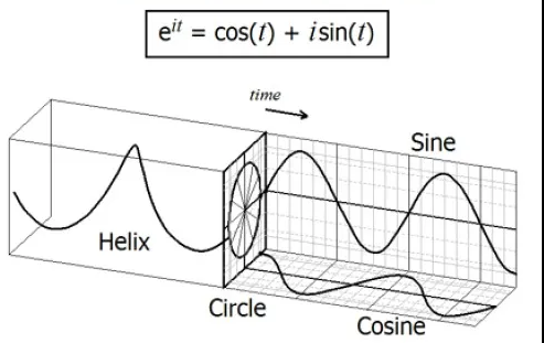
Visual representation of Euler’s formula in 3d space
Cooley-Tukey FFT algorithm
Now that we have the frequencies we want to convert this to something visual we can do this with the Inverse Fast Fourier Transform, which converts our frequency domain texture to the time domain.
The IFFT is an algorithm that efficiently computes the DFT(discrete Fourier transform) which makes it faster for real-time, since the DFT is used to transform signals from the time domain into the frequency domain we want to calculate it’s inverse.
The most common algorithm to calculate the FFT is the Cooley-Tukey algorithm and we use the radix-2 DIT case which is the simplest form of the algorithm. The algorithm divides a DFT of size N into two interleaved DFTs (hence the name “radix-2”) of size N/2 with each recursive stage (wikipedia), there are a total of log2(N) stages needed in order to transform the signal to the time domain. In our case N is the size of our texture 512x512px.
For this algorithm we need to sort the data so that the even and odd numbers are grouped together we do this by doing a binary reversal on the index of the pixel so px1, px2, …, after reversing the binaries we simply count up the binary numbers and we are left with the first half being even numbers and the second half being odd.
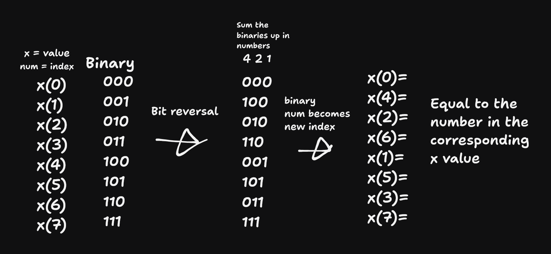
Now that we have the data ordered correctly we have one last step left, and that is calculating the DFTs. The algorithm gains its speed by re-using the results of intermediate computations to compute multiple DFT outputs. Note that final outputs are obtained by a +/− combination of $E_k \text{ and } O_k \exp\left(-\frac{2\pi i k}{N}\right)$
| $E_k$ | means even number, and k is the index. |
| $O_k$ | means on even number, and k is the index. |
| $N$ | is the size of the texture. |
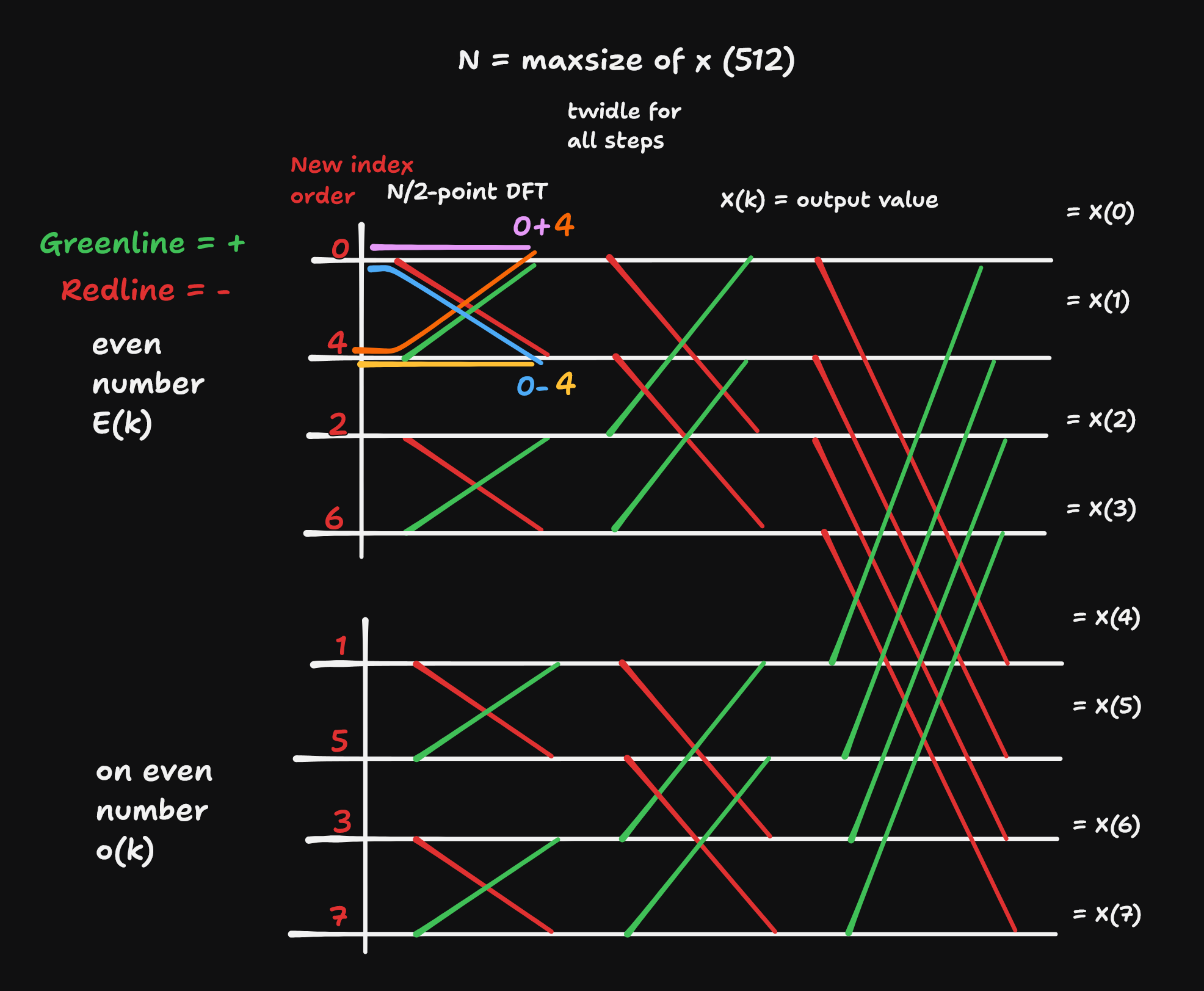
FFT butterfly computations for 8 pixel texture
The image shows a rough structure of how it would look like for an 8 texture size but in our case it would be a lot bigger with a 512 texture size. We calculate a total of 5 IFFT 3 for the displacement and 2 IFFT for the slope map which is calculated with the derivatives.
It is not necessary to know how it exactly works but If you are looking for an even more in depth explanation I would recommend watching this video
Creating a displacement and slope map
The last step is to create 2 textures 1 texture for the vertices displacement and a slope map which will be used for the normals. We arranged the data before our calculation in a way that is ideal for the Cooley-Tukey algorithm but this results in a weird looking texture since the data is not in the correct order.
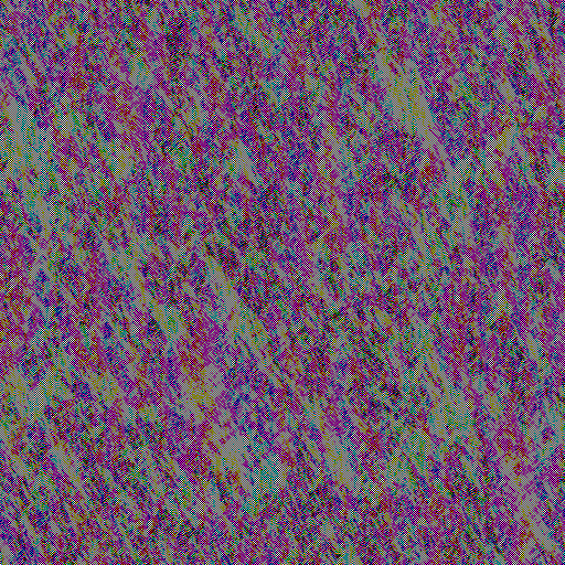
slope texture before permute
To fix this we need to permute the data according to the pixel id. After storing everything inside the texture we will be left with 2 textures.
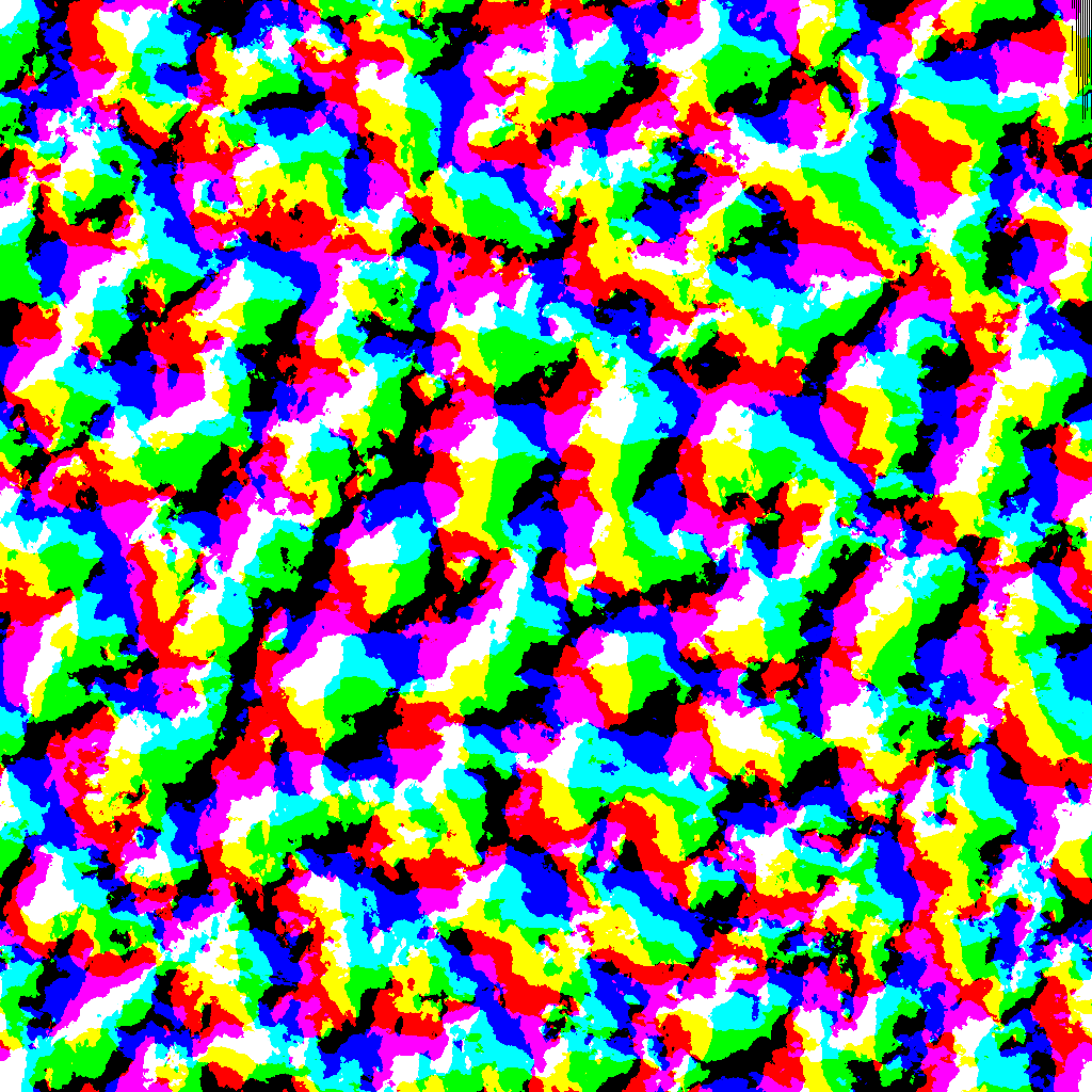
Final displacement map
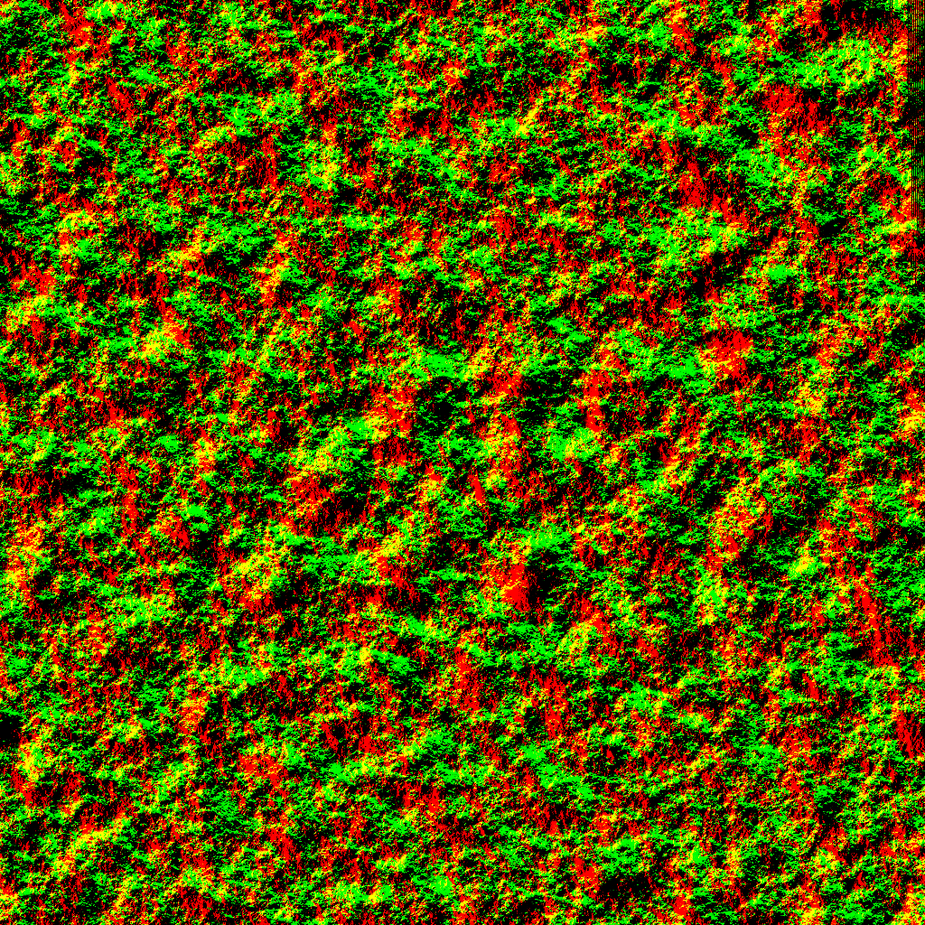
Final slope map
How to apply these texture in practice
We simply apply the displacement textures values before we transform our position to world space.
// pseudo code
float3 diplacement = sample.(DisplacementMap).xyz

out.pos += diplacement;

// out.pos to world space
And for the normals we sample the slope map like this
// pseudo code
float3 normal = sample.(slopemap).xyz

// The slope map consist of only 2 IFFT so this mean it only has 2 values
normal = normalize(float3(-normals.x, 1.0f, -normals.y));
// y becomes the z of the normal since y will always be up unless you engine is structured differently
Shading
I feel like it is also important to talk a little bit about how these games shade their water since they are not just using your average PBR shader they are also including environmental reflections and light scattering, in a GDC talk from the developers of Atlas they talk about this in high detail.
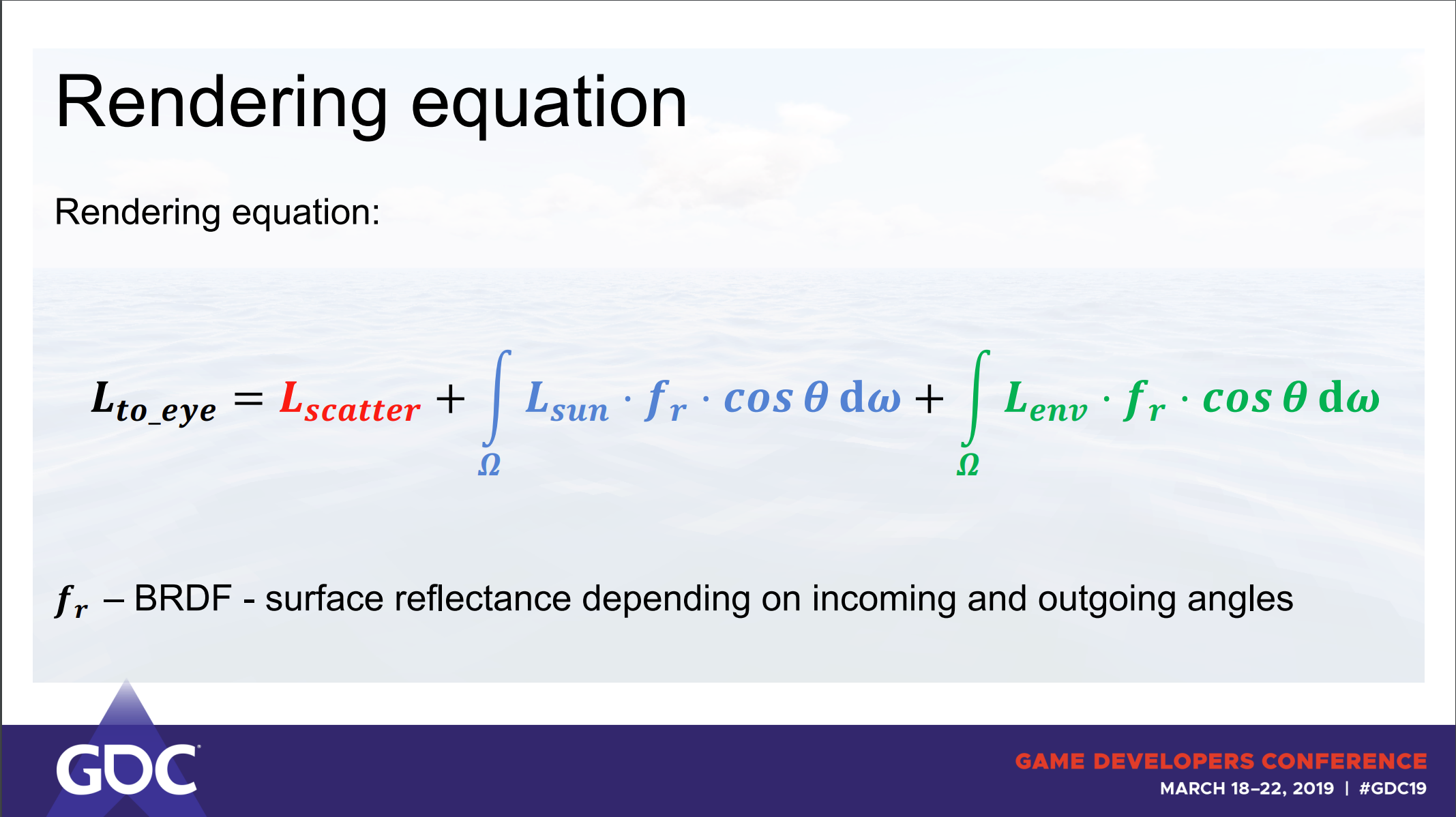
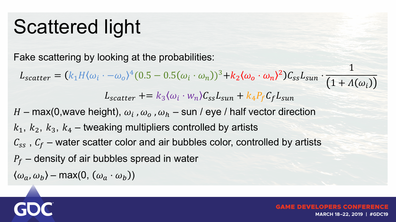
In short they talk about approximating light scattering through the wave since it would be to expensive to calculate it accurately. The fake scattering by using the formula bellow
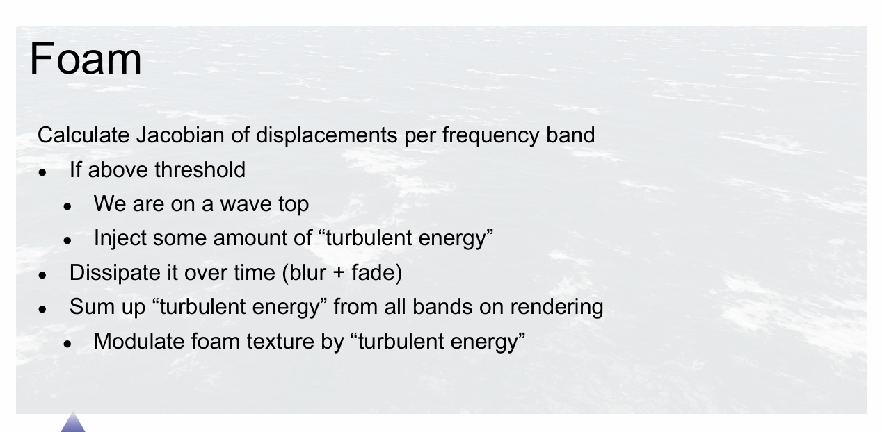
Atlas also talks a little bit about foam where they calculate the Jacobian of the displacement with this calculation u can see where the amplitude of the weaves curls over if it curls over we apply a blur and fade to the foam, for convenience sake we store this in the displacements alpha channel.
Final result
Optimizations
There are multiple optimizations we can do which will mainly be focused on the amount of vertices visible we can do a simple CPU frustum culling which will work for most type of games where only a small part of the ocean is visible at a time. This works by having an AABB bound for each tile, so the bottom left position of the tile and the top right position of the tile, if they are in the view frustum they will be drawn otherwise not.
Beside adding frustum culling the performance would also greatly benefit from adding tessellation this will give more vertices/detail up close and display less vertices further away where everything doesn’t need as much detail.
Future improvement
There are still a lot of things we can improve upon like:
- Adding filtering for texture so everything looks less pixelated
- Adding tessellation for better performance
- Having buoyancy so ships and objects can float
- Adding wakes and water displacement
- A simple distance fog
- A post process filter for when the camera is under the waves
- Fixing the tiling issues
- Adding particle splash effects on wave collision
Conclusion
I hope I gave a good inside, on how some of these big studios might have implemented realistic oceans in their games and what steps you could follow to get the basics of a realistic looking water implementation running, and as you can see above there are still a lot of improvements we can make in the future to make it more interactable which sell’s the illusion even more.
I hope this article was helpful in giving a good insight on this topic and if there is anything you still have questions on just send an e-mail to 230160@buas.nl.
Here are some valuable resources that greatly help me creating my final product:
- Simulating ocean water - Jerry Tessendorf
- Wakes, explosions and lighting interactive water simulation in Atlas
- Ocean waves simulation with Fast Fourier transform - Jump Trajectory This was a big inspiration for making the project
- konstantinkz.github.io/water-rendering-tutorial/ Great blog which gave a good explanation on the shading module of the water
- Simulating the entire ocean - Acerola
- Ocean-Wave Spectra - wiki waves
This blog post was created by Jim van der Heijden, in my second year as a student of the Creative Media and Game Technologies course at Breda University of Applied Sciences.
